Most delays take some inflow, shift it in time, and smooth it out. As we saw in the first section the higher order the delay the less smoothing occurs. In some cases, however, you might want a smooth inflow to be broken up into batches, and this is what DELAY BATCH does.
Consider the production of pottery in a facility with a single large kiln. A typical continuous representation of this would be a structure such as (batch1.mdl):

Here firing is given by the equation:
| firing= | MIN(kiln capacity/firing time, |
| Formed Unfired Pottery/firing time) |
However, if the kiln loaded, then started it is more accurate to represent the model with a batch process (batch2.mdl):

Now the equation for firing is:
| firing= | DELAY BATCH(sporadic forming, kiln capacity, |
firing time, 0, 0, 0)
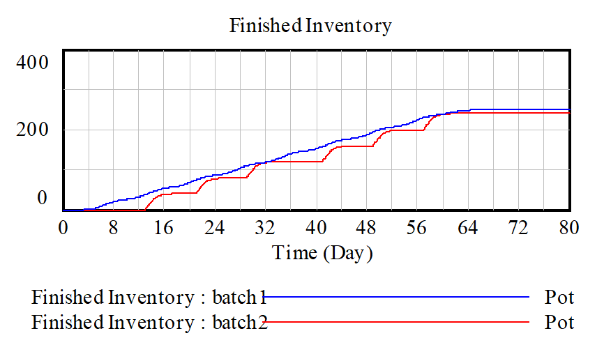
The final output is much more episodic, though not too much different:

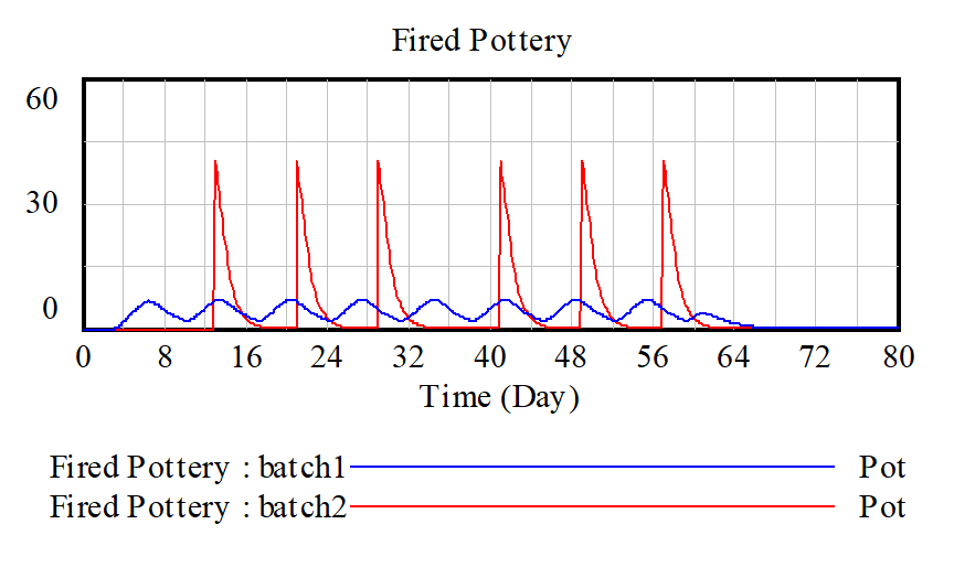
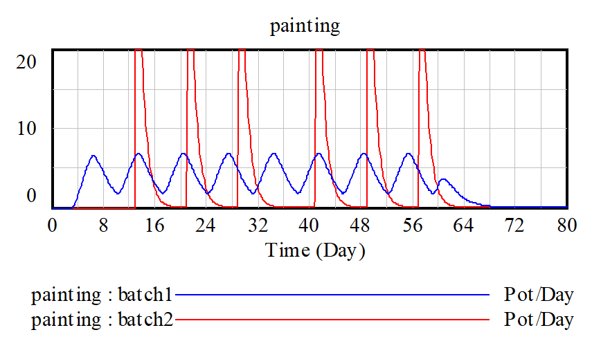
but there is a much bigger variation in the amount of fired pottery and consequently in the level of painting activity.


In situations where real activities are episodic and the capacity constraints tend to be limiting during those episodes using the DELAY BATCH function can give more accurate results.